Qubit-Efficient Encoding Techniques for Solving QUBO Problems

🧠 Introduction

Classical algorithms are already incredibly effective at solving many optimization problems — especially when the number of variables is in the low thousands. However, when scaling up to problems involving tens or hundreds of thousands of binary variables, classical solvers begin to falter due to the combinatorial explosion in the search space.

Quantum computing offers a compelling alternative — not by brute force, but by exploring exponentially large solution spaces in parallel using quantum superposition and entanglement. One popular quantum algorithm for such problems is the Quantum Approximate Optimization Algorithm (QAOA) [3], a textbook example of a variational quantum algorithm (VQA). However, QAOA requires one qubit per binary variable, which becomes prohibitively resource-intensive for large-scale problems.

For instance, solving a QUBO (Quadratic Unconstrained Binary Optimization) problem with 10,000 variables using QAOA would require 10,000 logical qubits — a scale far beyond current quantum hardware capabilities.

🔍 Why Qubit-Efficient Methods?

This demo explores qubit-efficient alternatives to QAOA that are not only suitable for today’s NISQ (Noisy Intermediate-Scale Quantum) devices, but also generalizable across combinatorial optimization problems.

We specifically demonstrate these methods in the context of unsupervised image segmentation, by:

1. Formulating segmentation as a min-cut problem over a graph derived from the image.
2. Reformulating the min-cut as a QUBO problem.
3. Solving the QUBO using qubit-efficient VQAs, namely [1]:
   • Parametric Gate Encoding (PGE)
   • Ancilla Basis Encoding (ABE)
   • Adaptive Cost Encoding (ACE)

These methods only require a logarithmic number of qubits with respect to the problem size (i.e., number of binary variables). This makes them scalable and implementable even on near-term quantum hardware. Moreover, the exact graph-based image segmentation technique have been explored also using quantum annealers [2].

While this demo walks through an image segmentation example, the encoding schemes presented here can be applied to any binary combinatorial optimization problem.

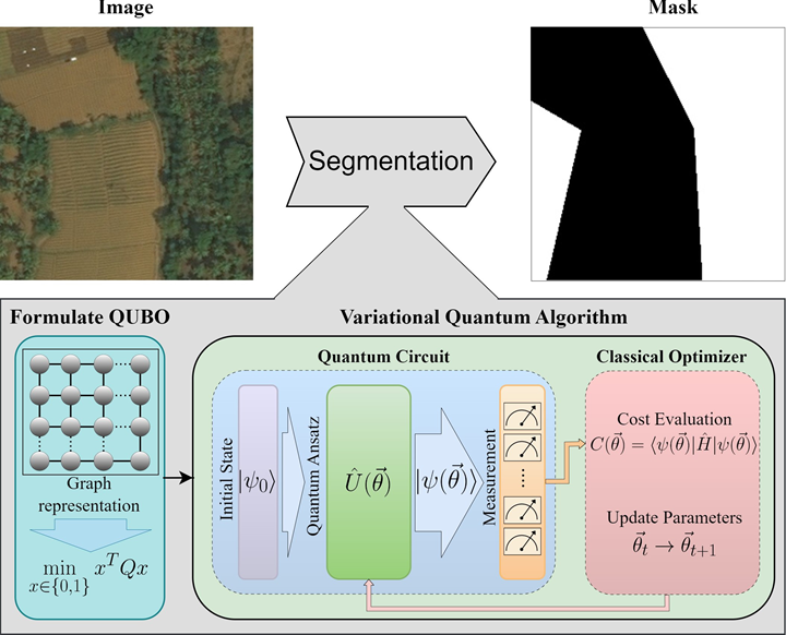
Architecture for segmenting an image by transforming it into a graph and solving the corresponding minimum cut as a QUBO problem using variational quantum circuits [1]

Clone the Repository: Begin by cloning the repository to your local machine. Open a terminal/cmd/powershell and run

   git clone https://github.com/supreethmv/Pennylane-ImageSegmentation.git
   cd Pennylane-ImageSegmentation

Install Dependencies: Use the provided requirements.txt to install all necessary libraries. The process may take a few minutes depending on your internet speed and the packages already available in your system.

   pip install -r requirements.txt

Open a jupyter notebook and execute the below python code.

🧱 Import dependencies

We begin by importing the standard Python libraries for graph construction and visualization, and PennyLane modules for quantum circuit construction and simulation. This setup ensures a seamless interface for hybrid quantum-classical processing.

import numpy as np
import networkx as nx
import pennylane as qml
from scipy.optimize import minimize, differential_evolution
import matplotlib.pyplot as plt

from math import ceil, log2
import time

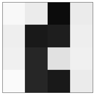
🖼️ Generate an Example Image

To keep things intuitive, we generate a toy grayscale image. This synthetic image will be segmented using quantum algorithms.

We use a simple 4×4 grid for clarity. The pixel intensities will act as a proxy for similarity when we later construct a graph. Each pixel becomes a vertex, and edges represent similarity (e.g., inverse of intensity difference).

height,width = 4,4
image = np.array([
       [0.97,  0.92, 0.05, 0.92],
       [0.93,  0.10, 0.12, 0.93],
       [0.94,  0.15, 0.88, 0.94],
       [0.98,  0.15, 0.10, 0.92]
       ])


plt.imshow(image, interpolation='nearest', cmap=plt.cm.gray, vmin=0, vmax=1)
# plt.axis('off')
plt.xticks([])
plt.yticks([])
plt.show()

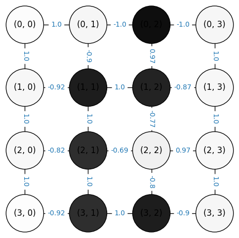
🔗 Representing Image as a Graph

Each image is modeled as an undirected weighted grid graph:

• Each pixel becomes a node.
• An edge exists between neighboring pixels.
• The weight reflects similarity (e.g., inverse absolute difference in grayscale values).

This transforms the segmentation task into a minimum cut problem, where the goal is to partition the graph to minimize the sum of cut edge weights.

def image_to_grid_graph(gray_img, sigma=0.5):
  # Convert image to grayscale
  h, w = gray_img.shape
  # Initialize graph nodes and edges
  nodes = np.zeros((h*w, 1))
  edges = []
  nx_elist = []
  # Compute node potentials and edge weights
  min_weight = 1
  max_weight = 0
  for i in range(h*w):
    x, y = i//w, i%w
    nodes[i] = gray_img[x,y]
    if x > 0:
      j = (x-1)*w + y
      weight = 1-np.exp(-((gray_img[x,y] - gray_img[x-1,y])**2) / (2 * sigma**2))
      edges.append((i, j, weight))
      nx_elist.append(((x,y),(x-1,y),np.round(weight,2)))
      if min_weight>weight:min_weight=weight
      if max_weight<weight:max_weight=weight
    if y > 0:
      j = x*w + y-1
      weight = 1-np.exp(-((gray_img[x,y] - gray_img[x,y-1])**2) / (2 * sigma**2))
      edges.append((i, j, weight))
      nx_elist.append(((x,y),(x,y-1),np.round(weight,2)))
      if min_weight>weight:min_weight=weight
      if max_weight<weight:max_weight=weight
  a=-1
  b=1
  if max_weight-min_weight:
    normalized_edges = [(node1,node2,-1*np.round(((b-a)*((edge_weight-min_weight)/(max_weight-min_weight)))+a,2)) for node1,node2,edge_weight in edges]
    normalized_nx_elist = [(node1,node2,-1*np.round(((b-a)*((edge_weight-min_weight)/(max_weight-min_weight)))+a,2)) for node1,node2,edge_weight in nx_elist]
  else:
    normalized_edges = [(node1,node2,-1*np.round(edge_weight,2)) for node1,node2,edge_weight in edges]
    normalized_nx_elist = [(node1,node2,-1*np.round(edge_weight,2)) for node1,node2,edge_weight in nx_elist]
  return nodes, edges, nx_elist, normalized_edges, normalized_nx_elist

pixel_values, elist, nx_elist, normalized_elist, normalized_nx_elist = image_to_grid_graph(image)

pixel_values, normalized_nx_elist

(array([[0.97],
        [0.92],
        [0.05],
        [0.92],
        [0.93],
        [0.1 ],
        [0.12],
        [0.93],
        [0.94],
        [0.15],
        [0.88],
        [0.94],
        [0.98],
        [0.15],
        [0.1 ],
        [0.92]]),
 [((0, 1), (0, 0), np.float64(1.0)),
  ((0, 2), (0, 1), np.float64(-1.0)),
  ((0, 3), (0, 2), np.float64(-1.0)),
  ((1, 0), (0, 0), np.float64(1.0)),
  ((1, 1), (0, 1), np.float64(-0.9)),
  ((1, 1), (1, 0), np.float64(-0.92)),
  ((1, 2), (0, 2), np.float64(0.97)),
  ((1, 2), (1, 1), np.float64(1.0)),
  ((1, 3), (0, 3), np.float64(1.0)),
  ((1, 3), (1, 2), np.float64(-0.87)),
  ((2, 0), (1, 0), np.float64(1.0)),
  ((2, 1), (1, 1), np.float64(1.0)),
  ((2, 1), (2, 0), np.float64(-0.82)),
  ((2, 2), (1, 2), np.float64(-0.77)),
  ((2, 2), (2, 1), np.float64(-0.69)),
  ((2, 3), (1, 3), np.float64(1.0)),
  ((2, 3), (2, 2), np.float64(0.97)),
  ((3, 0), (2, 0), np.float64(1.0)),
  ((3, 1), (2, 1), np.float64(1.0)),
  ((3, 1), (3, 0), np.float64(-0.92)),
  ((3, 2), (2, 2), np.float64(-0.8)),
  ((3, 2), (3, 1), np.float64(1.0)),
  ((3, 3), (2, 3), np.float64(1.0)),
  ((3, 3), (3, 2), np.float64(-0.9))])

G = nx.grid_2d_graph(image.shape[0], image.shape[1])
G.add_weighted_edges_from(normalized_nx_elist)

def draw(G):
  plt.figure(figsize=(6,6))
  default_axes = plt.axes(frameon=True)
  pos = {(x,y):(y,-x) for x,y in G.nodes()}
  nx.draw_networkx(G, pos)
  nodes = nx.draw_networkx_nodes(G, pos, node_color=1-pixel_values,
                  node_size=3000,
                  cmap=plt.cm.Greys, vmin=0, vmax=1)
  nodes.set_edgecolor('k')
  edge_labels = nx.get_edge_attributes(G, "weight")
  nx.draw_networkx_edge_labels(G,
                              pos=pos,
                              edge_labels=edge_labels,
                              font_size=10,
                              font_color='tab:blue')
  plt.axis('off')
draw(G)
plt.show()

🔁 Parametric Gate Encoding (PGE)

In PGE, we directly encode the binary segmentation mask in the rotation parameters of a diagonal gate [4].

Only $\log_2(n)$ qubits are required, which is a huge gain over methods like QAOA that need $O(n)$.

Quantum Circuit:

• Apply Hadamard gates to initialize a uniform superposition.
• Apply a diagonal gate $U(\vec{\theta})$ whose entries encode binary values using a thresholding function $f(\theta_i)$.
• Evaluate the cost function: \(C(\vec{\theta}) = \langle \psi(\vec{\theta}) | L_G | \psi(\vec{\theta}) \rangle\) where $L_G$ is the graph Laplacian.

The result is optimized using a classical optimizer, and $\theta_i$ are mapped to bits depending on whether $\theta_i < \pi$ or not.

n = G.number_of_nodes()
n_qubits = int(np.ceil(np.log2(n)))
n_qubits

def R(theta): 
    if abs(theta) > 2*np.pi or abs(theta) < 0:
        theta = abs(theta) - (np.floor(abs(theta)/(2*np.pi))*(2*np.pi))
    return 0 if 0 <= theta < np.pi else 1

# Define a PennyLane quantum device (using default.qubit simulator)
dev = qml.device("default.qubit", wires=n_qubits)

# Quantum circuit as a QNode
@qml.qnode(dev)
def circuit(params, H):
    # N = len(params)
    N = int(np.log2(len(params)))
    for i in range(N):
        qml.Hadamard(wires=i)
    
    diagonal_elements = [np.exp(1j * np.pi * R(param)) for param in params]
    # qml.DiagonalQubitUnitary(np.diag(diagonal_elements), wires=list(range(N)))
    qml.DiagonalQubitUnitary(diagonal_elements, wires=list(range(N)))
    
    return qml.expval(qml.Hermitian(H, wires=list(range(N))))

def cost_fn(params, H):
    global optimization_iteration_count
    optimization_iteration_count += 1
    cost = circuit(params, H)
    print(f'@ Iteration {optimization_iteration_count} Cost :', cost)
    return cost

def decode(optimal_params):
    return [R(param) for param in optimal_params]

def objective_value(x, w):
    return np.dot(x, np.dot(w, x))

def new_nisq_algo_solver(G, optimizer_method='Powell', initial_params_seed=123):
    global optimization_iteration_count
    optimization_iteration_count = 0
    n = G.number_of_nodes()
    w = nx.adjacency_matrix(G).todense()
    D_G = np.diag(list(dict(G.degree()).values()))
    A_G = w
    L_G = D_G - A_G
    n_padding = (2**int(np.ceil(np.log2(n)))-n)
    L_G = np.pad(L_G, [(0, n_padding), (0, n_padding) ], mode='constant')
    H = L_G
    
    np.random.seed(seed=initial_params_seed)
    initial_params = np.random.uniform(low=0.5, high=2*np.pi , size=(n+n_padding))
    
    result = minimize(
        fun=cost_fn,
        x0=initial_params,
        args=(H,),
        method=optimizer_method,
    )
    
    optimal_params, expectation_value = result.x, result.fun
    x = np.real(decode(optimal_params))
    x = x[:n]
    cut_value = objective_value(x, w)
    
    return x, expectation_value, cut_value

binary_solution, expectation_value, cut_value = new_nisq_algo_solver(G, optimizer_method = 'Powell')
binary_solution, expectation_value, cut_value

@ Iteration 1 Cost : 2.7137499999999983
@ Iteration 2 Cost : 2.7137499999999983
@ Iteration 3 Cost : 2.7137499999999983
@ Iteration 4 Cost : 2.7137499999999983
@ Iteration 5 Cost : 2.7137499999999983
.
.
.
@ Iteration 349 Cost : 0.18374999999999986
@ Iteration 350 Cost : 0.18374999999999986
@ Iteration 351 Cost : 0.18374999999999986
@ Iteration 352 Cost : 0.18374999999999986
@ Iteration 353 Cost : 0.18374999999999986

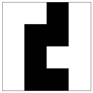
def decode_binary_string(x, height, width):
  mask = np.zeros([height, width])
  for index,segment in enumerate(x):
    mask[index//width,index%width]=segment
  return mask

mask = decode_binary_string(binary_solution, height, width)
plt.imshow(mask, interpolation='nearest', cmap=plt.cm.gray, vmin=0, vmax=1)
plt.xticks([])
plt.yticks([])
plt.show()

🧪 Ancilla Basis Encoding (ABE)

ABE uses $\log_2(n) + 1$ qubits:

• $\log_2(n)$ register qubits represent binary states.
• One ancilla qubit helps encode the binary decision.

Each computational basis state of the register corresponds to one binary variable. The ancilla qubit’s amplitude is used to decide the bit value ^[5]: \(x_{v_i} = \begin{cases} 0 & \text{if } |a_i|^2 > |b_i|^2 \\ 1 & \text{otherwise} \end{cases}\)

The cost function is parameterized over expectation values of basis state projectors: \(C(\vec{\theta}) = \sum_{i,j} Q_{ij} \frac{\langle \hat{P}_i^1 \rangle \langle \hat{P}_j^1 \rangle}{\langle \hat{P}_i \rangle \langle \hat{P}_j \rangle} (1 - \delta_{ij}) + \sum_i Q_{ii} \frac{\langle \hat{P}_i^1 \rangle}{\langle \hat{P}_i \rangle}\)

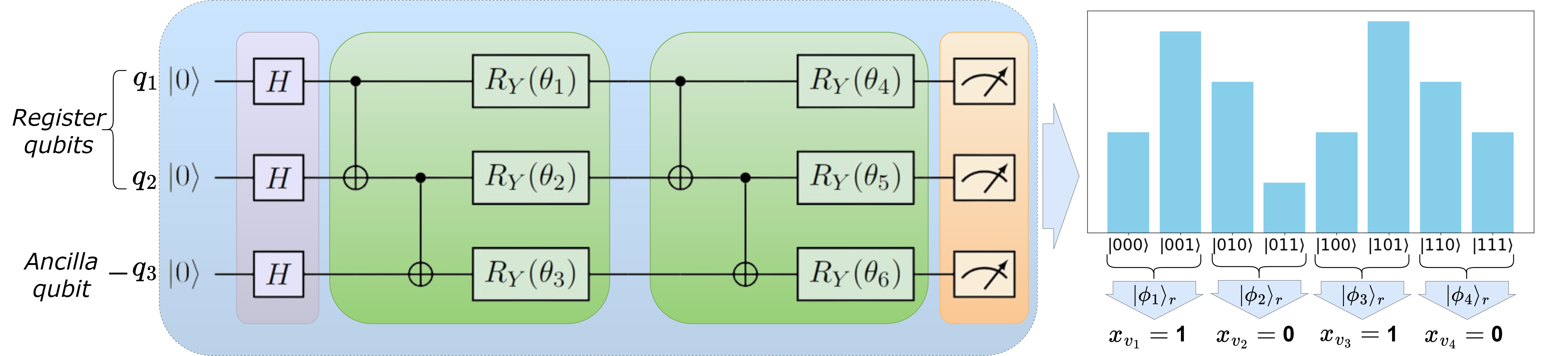Example of a quantum circuit of ABE/ACE for solving QUBO of size 4 using 3 qubits (2 register + 1 ancilla), whereas in this demo we are solving a QUBO of size 16, so we are simulating 5 qubits. Basis state amplitudes are used to decode the binary solution (Fig. 3 in [1]

def get_qubo_matrix(W):
    """Computes the QUBO matrix for the Minimum Cut problem given a weight matrix W."""
    n = W.shape[0]  # Number of nodes
    Q = np.zeros((n, n))  # Initialize QUBO matrix
    
    for i in range(n):
        Q[i, i] = np.sum(W[i])  # Diagonal terms (degree of node)
        for j in range(n):
            if i != j:
                Q[i, j] = -W[i, j]  # Off-diagonal terms (negative adjacency)
    
    return Q

def get_circuit(nq, n_layers):
    def circuit(params):
        for i in range(nq):
            qml.Hadamard(wires=i)
        for layer_i in range(n_layers):
            for qubit_i in range(nq - 1):
                qml.CNOT(wires=[qubit_i, (qubit_i + 1) % nq])
            for qubit_i in range(nq):
                qml.RY(params[(nq * layer_i) + qubit_i], wires=qubit_i)
        return qml.probs(wires=range(nq))
    return circuit

def get_projectors(probabilities, n_c):
    P, P1 = [0] * n_c, [0] * n_c
    for k, v in probabilities.items():
        index = int(k[1:], 2)
        P[index] += v
        if k[0] == '1':
            P1[index] += v
    return P, P1

def objective_value(x, w):
    return sum(w[i, j] * x[i] * (1 - x[j]) for i in range(len(x)) for j in range(len(x)))

def decode_probabilities(probabilities):
    binary_solution, n_r = [], len(list(probabilities.keys())[0]) - 1
    for i in range(2**n_r):
        zero_state, one_state = '0' + format(i, 'b').zfill(n_r), '1' + format(i, 'b').zfill(n_r)
        if zero_state in probabilities and one_state in probabilities:
            binary_solution.append(0 if probabilities[zero_state] > probabilities[one_state] else 1)
        elif zero_state in probabilities:
            binary_solution.append(0)
        elif one_state in probabilities:
            binary_solution.append(1)
    return binary_solution

def evaluate_cost(params, circuit, qubo_matrix):
    global valid_probabilities, optimization_iteration_count, best_cost, best_params
    optimization_iteration_count += 1
    raw_probs = circuit(params)  # NumPy array

    # Convert probability array to dictionary with bitstrings
    num_qubits = int(np.log2(len(raw_probs)))
    bitstrings = [format(i, f'0{num_qubits}b') for i in range(len(raw_probs))]
    probabilities = {bitstrings[i]: raw_probs[i] for i in range(len(raw_probs))}
    
    n_c = 2**(len(bitstrings[0])-1)
    P, P1 = get_projectors(probabilities, n_c)
    if 0 in P:
        return float("inf")

    valid_probabilities = probabilities.copy()
    cost = sum(qubo_matrix[i][j] * P1[i] / P[i] if i == j else (qubo_matrix[i][j] * P1[i] * P1[j]) / (P[i] * P[j])
               for i in range(len(qubo_matrix)) for j in range(len(qubo_matrix)))
    
    # Track the best cost and parameters manually
    if cost < best_cost:
        best_cost = cost
        best_params = params.copy()  # Store the best parameter set
    
    print(f'@ Iteration {optimization_iteration_count} Cost :', cost)
    return cost

def ancilla_basis_encoding(G, initial_params, n_layers=1, optimizer_method='differential_evolution'):
    w = nx.adjacency_matrix(G).todense()
    Q = get_qubo_matrix(W = w)
    nc, nq = len(G.nodes()), ceil(log2(len(G.nodes()))) + 1
    dev = qml.device("default.qubit", wires=nq, shots=None)
    qnode = qml.QNode(get_circuit(nq, n_layers), dev)
    global valid_probabilities, optimization_iteration_count, best_cost, best_params  # Track the best parameters
    valid_probabilities, optimization_iteration_count = [], 0
    best_cost = float("inf")  # Initialize best cost
    best_params = None  # Initialize best parameters
    if optimizer_method == "differential_evolution":
        optimization_result = differential_evolution(
            func=evaluate_cost,
            bounds=[(-np.pi, np.pi)] * len(initial_params),
            args=(qnode, Q),
            strategy='best1bin',
            maxiter=100,
            popsize=15
        )
    else:
        optimization_result = minimize(fun=evaluate_cost, x0=initial_params, args=(qnode, Q), method=optimizer_method,
                                       bounds=[(-np.pi, np.pi)] * len(initial_params))
    if not valid_probabilities:
        return False, [0] * nc, 0, 0, [0] * len(initial_params)
    best_raw_probs = qnode(best_params)
    bitstrings = [format(i, f'0{nq}b') for i in range(len(best_raw_probs))]
    best_probabilities = {bitstrings[i]: best_raw_probs[i] for i in range(len(best_raw_probs))}
    binary_solution = decode_probabilities(best_probabilities)[:nc]
    print("binary_solution",binary_solution)
    return binary_solution, best_cost, objective_value(np.array(binary_solution), w), best_params

Although the code can handle various methods available in scipy.minimize, in this demo we will be using a more robust genetic algorithm differential_evolution as the classical optimizer.

initial_params_seed, scipy_optimizer_method, n_layers = 1234, "differential_evolution", 5
nq = ceil(log2(len(G.nodes()))) + 1
np.random.seed(initial_params_seed)
initial_params = np.random.uniform(low=-np.pi, high=np.pi, size=nq * n_layers)
print(f"Executing QC with {n_layers} layers and {scipy_optimizer_method} optimizer.")
start_time = time.time()
solution, value, cut_value, optimal_params = ancilla_basis_encoding(G, initial_params, n_layers, scipy_optimizer_method)
end_time = time.time()
print(solution, value, cut_value, optimal_params)

mask = decode_binary_string(solution, height, width)
plt.imshow(mask, interpolation='nearest', cmap=plt.cm.gray, vmin=0, vmax=1)
plt.xticks([])
plt.yticks([])
plt.show()

Executing QC with 5 layers and differential_evolution optimizer.
@ Iteration 1 Cost : 1.9517729104828314
@ Iteration 2 Cost : 2.695380482787284
@ Iteration 3 Cost : 1.2997220934905251
@ Iteration 4 Cost : 3.285955280870637
@ Iteration 5 Cost : 1.6088763974114462
.
.
.
@ Iteration 41615 Cost : -9.580055050943331
@ Iteration 41616 Cost : -9.580055063692425
@ Iteration 41617 Cost : -9.58005504857137
@ Iteration 41618 Cost : -9.58005504350123
@ Iteration 41619 Cost : -9.580055055239168
binary_solution [0, 0, 1, 0, 0, 1, 1, 0, 0, 1, 0, 0, 0, 1, 1, 0]
[0, 0, 1, 0, 0, 1, 1, 0, 0, 1, 0, 0, 0, 1, 1, 0] -9.580055070588434 -9.59 [-1.87128251 -1.26640308 -0.02336564 -3.10694607  0.01860386 -1.88002789
  0.51920146  3.11901893 -2.08946347  0.8140825  -1.68061883 -0.06049532
  1.8261264  -1.56490516 -0.5037992  -2.01992427 -0.42991677  1.15472694
  1.51827448  0.85008668  0.26731643  1.7789839   3.13530596  2.50698098
  1.62851782]

🔁 Adaptive Cost Encoding (ACE)

ACE modifies ABE by skipping the QUBO formulation entirely during evaluation.

Instead of optimizing over probabilities, we decode a binary vector $x$ from the measured output and evaluate the original min-cut cost function directly 1: \(C(x) = \sum_{i < j} x_i (1 - x_j) w(v_i, v_j)\)

This:

• Removes the need for a QUBO matrix, which can have loss of generality for constrained optimization problems when the penalty coefficient is not set appropriately.
• Improves convergence (the cost function is discrete and combinatorial).
• Aligns optimization directly with the true task objective.

def evaluate_cost_mincut(params, circuit, w):
    global valid_probabilities, optimization_iteration_count, best_cost, best_params
    optimization_iteration_count += 1
    raw_probs = circuit(params)  # NumPy array
    
    # Convert probability array to dictionary with bitstrings
    num_qubits = int(np.log2(len(raw_probs)))
    bitstrings = [format(i, f'0{num_qubits}b') for i in range(len(raw_probs))]
    probabilities = {bitstrings[i]: raw_probs[i] for i in range(len(raw_probs))}
    
    n_c = 2**(len(bitstrings[0])-1)
    P, P1 = get_projectors(probabilities, n_c)
    if 0 in P:
        return float("inf")
    valid_probabilities = probabilities.copy()
    binary_solution = decode_probabilities(valid_probabilities)[:len(w)]
    cost = objective_value(np.array(binary_solution), w)

    # Track the best cost and parameters manually
    if cost < best_cost:
        best_cost = cost
        best_params = params.copy()  # Store the best parameter set
    
    print(f'@ Iteration {optimization_iteration_count} Cost :', cost)
    return cost

def adaptive_cost_encoding_de(G, initial_params, n_layers=1, optimizer_method='differential_evolution'):
    w = nx.adjacency_matrix(G).todense()
    nc, nq = len(G.nodes()), ceil(log2(len(G.nodes()))) + 1
    dev = qml.device("default.qubit", wires=nq, shots=None)
    qnode = qml.QNode(get_circuit(nq, n_layers), dev)
    global valid_probabilities, optimization_iteration_count, best_cost, best_params  # Track the best parameters
    valid_probabilities, optimization_iteration_count = [], 0
    best_cost = float("inf")  # Initialize best cost
    best_params = None  # Initialize best parameters

    if optimizer_method == "differential_evolution":
        optimization_result = differential_evolution(
            func=evaluate_cost_mincut,
            bounds=[(-np.pi, np.pi)] * len(initial_params),
            args=(qnode, w),
            strategy='best1bin',
            maxiter=100,
            popsize=15
        )
    else:
        optimization_result = minimize(fun=evaluate_cost_mincut, x0=initial_params, args=(qnode, w), method=optimizer_method,
                                       bounds=[(-np.pi, np.pi)] * len(initial_params))
    
    if not valid_probabilities:
        return False, [0] * nc, 0, 0, [0] * len(initial_params)
    
    best_raw_probs = qnode(best_params)
    bitstrings = [format(i, f'0{nq}b') for i in range(len(best_raw_probs))]
    best_probabilities = {bitstrings[i]: best_raw_probs[i] for i in range(len(best_raw_probs))}
    binary_solution = decode_probabilities(best_probabilities)[:nc]
    print("binary_solution",binary_solution)
    return binary_solution, best_cost, objective_value(np.array(binary_solution), w), best_params

initial_params_seed, scipy_optimizer_method, n_layers = 1234, "differential_evolution", 5
nq = ceil(log2(len(G.nodes()))) + 1
np.random.seed(initial_params_seed)
initial_params = np.random.uniform(low=-np.pi, high=np.pi, size=nq * n_layers)
print(f"Executing QC with {n_layers} layers and Differential Evolution optimizer.")
start_time = time.time()
solution, value, cut_value, optimal_params = adaptive_cost_encoding_de(G, initial_params, n_layers, optimizer_method=scipy_optimizer_method)
end_time = time.time()
print(solution, value, cut_value, optimal_params)

mask = decode_binary_string(solution, height, width)
plt.imshow(mask, interpolation='nearest', cmap=plt.cm.gray, vmin=0, vmax=1)
plt.xticks([])
plt.yticks([])
plt.show()

Executing QC with 5 layers and Differential Evolution optimizer.
@ Iteration 1 Cost : 2.16
@ Iteration 2 Cost : 3.33
@ Iteration 3 Cost : 3.1799999999999997
@ Iteration 4 Cost : 3.6700000000000004
@ Iteration 5 Cost : 3.6199999999999997
.
.
.
@ Iteration 37897 Cost : -9.59
@ Iteration 37898 Cost : -9.59
@ Iteration 37899 Cost : -9.59
@ Iteration 37900 Cost : -9.59
@ Iteration 37901 Cost : -9.59
binary_solution [1, 1, 0, 1, 1, 0, 0, 1, 1, 0, 1, 1, 1, 0, 0, 1]
[1, 1, 0, 1, 1, 0, 0, 1, 1, 0, 1, 1, 1, 0, 0, 1] -9.59 -9.59 [ 1.5925252  -0.99312378 -0.3011605  -0.64446057 -0.11583278  0.92450533
  1.92449243  0.57549626  0.32784236  1.36375091  0.64730511  0.85830076
 -2.96974057  1.52604576 -0.36825457  1.44591007  2.30640898 -2.26932841
  0.11814597  0.55094776  0.13729049 -2.39043552 -1.73403799 -1.58710222
  2.56579511]

📈 Evaluation & Observations

• PGE has a compact circuit but many parameters.
• ABE introduces a more efficient encoding at the cost of probabilistic decoding.
• ACE improves convergence by using the real problem cost and avoiding indirect probability-based objectives.

Theoretical scaling advantages:

• Qubit requirement is $O(\log n)$.
• Parametric gates and depth grow modestly with problem size.

Here’s the complexity comparison of QAOA, PGE, and ABE/ACE in terms of quantum resources for solving QUBO problems.

Method	Qubit Complexity	Entanglement Gates	Parametric Gates	Circuit Depth
QAOA	O(n)	O(n²)	O(L·n)	O(L·n²)
PGE	log₂(n)	n − 1	n	n
ABE / ACE	log₂(n) + 1	L·log₂(n)	L·(log₂(n) + 1)	L·(log₂(n) + 1)

(L is the ansatz depth, n is the number of QUBO variables.)

📎 Final Notes

This demo showcases scalable, qubit-efficient strategies for quantum-enhanced image segmentation.

By formulating image segmentation as a graph cut, reducing it to a QUBO, and then solving with advanced encodings like PGE, ABE, and ACE, we show that near-term quantum devices can tackle meaningful vision tasks.

---

📄 References

[1] S. M. Venkatesh, A. Macaluso, M. Nuske, M. Klusch, and A. Dengel, “Qubit-Efficient Variational Quantum Algorithms for Image Segmentation,” 2024 IEEE International Conference on Quantum Computing and Engineering (QCE), Montreal, QC, Canada, 2024, pp. 450–456. DOI: 10.1109/QCE60285.2024.00059, arXiv:2405.14405

[2] S. M. Venkatesh, A. Macaluso, M. Nuske, M. Klusch and A. Dengel, “Q-Seg: Quantum Annealing-Based Unsupervised Image Segmentation,” in IEEE Computer Graphics and Applications, vol. 44, no. 5, pp. 27-39, Sept.-Oct. 2024, doi: 10.1109/MCG.2024.3455012, arXiv:2311.12912.

[3] Farhi, E., Goldstone, J., & Gutmann, S. (2014). A quantum approximate optimization algorithm. arXiv preprint arXiv:1411.4028.

[4] Rančić, M. J. (2023). Noisy intermediate-scale quantum computing algorithm for solving an n-vertex MaxCut problem with log (n) qubits. Physical Review Research, 5(1), L012021. DOI: 10.1103/PhysRevResearch.5.L012021

[5] Tan, B., Lemonde, M. A., Thanasilp, S., Tangpanitanon, J., & Angelakis, D. G. (2021). Qubit-efficient encoding schemes for binary optimisation problems. Quantum, 5, 454. DOI: 10.22331/q-2021-05-04-454