Quantum-Powered Asset Clustering: Correlation Clustering with GCS-Q
A step-by-step guide to clustering financial assets using signed correlation graphs and quantum annealing with the GCS-Q algorithm.
Introduction
Portfolio managers and quantitative analysts spend a great deal of effort trying to understand how financial assets move together. If two stocks go up and down in near lockstep, holding both does little for diversification. Conversely, assets that move in opposite directions can hedge one another. The standard tool for quantifying these co-movements is the Pearson correlation coefficient, which yields values in $[-1, 1]$: a value near $+1$ means the two assets are highly correlated, near $-1$ means they are anticorrelated, and near $0$ means they are essentially uncorrelated.
A natural next step is to cluster assets into groups such that intra-cluster correlations are high (the assets in each group move together) and inter-cluster correlations are low or negative (different groups capture different market factors). This is the asset clustering problem, and it lies at the heart of:
- Portfolio optimization — Markowitz mean-variance optimization [5] benefits from well-separated clusters, since each cluster represents a distinct risk-return profile.
- Statistical arbitrage — pairs or basket trading strategies rely on identifying groups of cointegrated or highly correlated assets [6].
- Risk management — understanding correlation structures helps quantify systemic risk and contagion.
Why Classical Methods Struggle
Classical clustering algorithms such as $k$-Means, $k$-Medoids (PAM), hierarchical clustering, and even spectral methods like SPONGE [7] face four fundamental limitations when applied to signed correlation graphs:
(i) Number of clusters $k$ is not known in advance
Most classical methods require the user to specify $k$ before running the algorithm. In practice, the “right” number of clusters in a correlation matrix is unknown and changes over time as market regimes shift. Heuristics like the elbow method, silhouette analysis, or the eigengap criterion are expensive, data-dependent, and do not generalize across datasets.
(ii) Reformulation is lossy
Since classical methods require a positive-definite distance metric, Pearson correlations ($\rho \in [-1, 1]$) must be transformed into non-negative distances via mappings such as:
\[d_{ij}^{(\alpha)} = \sqrt{\alpha(1 - \rho_{ij})}, \quad \alpha > 0\]While this preserves ranking, it loses semantic fidelity. For example, a zero correlation $\rho_{ij} = 0$ (no relationship) maps to $\sqrt{\alpha}$, falsely implying a fixed non-zero dissimilarity. The rich signed structure of the original correlation graph is irreversibly discarded.
(iii) Optimization objective is different
Centroid-based methods (e.g., $k$-Means, PAM) optimize a proxy objective — minimizing distances to cluster centroids — rather than the true objective of maximizing intra-cluster correlations and minimizing inter-cluster correlations. Even when the distance transformation is applied, optimally solving the transformed problem does not recover the optimal clustering under the original signed graph.
(iv) Not robust for varying-sized clusters
Spectral methods like SPONGE perform well on sparse graphs with discrete weights $\in {-1, 0, +1}$ and approximately equal cluster sizes, but degrade significantly on dense financial correlation graphs with continuous weights and heterogeneous cluster structures. Similarly, $k$-Means assumes spherical, equally-sized clusters — an assumption that rarely holds in practice.
Enter GCS-Q
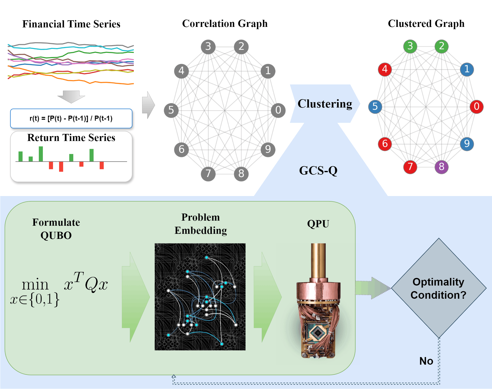
The Graph-based Coalition Structure Generation algorithm (GCS-Q) [3] was originally developed for cooperative game theory but is a natural fit for signed graph clustering. It operates directly on the signed, weighted correlation graph, avoiding lossy distance transformations. Starting with all assets in a single cluster, it recursively bipartitions each subgraph by solving a minimum-cut formulated as a QUBO (Quadratic Unconstrained Binary Optimization) problem, which is solved using a D-Wave quantum annealer. The algorithm automatically determines $k$, terminating when no further split improves intra-cluster agreement.
This post walks through the entire pipeline, from downloading stock data to running GCS-Q on D-Wave hardware, step by step.
Overview of the GCS-Q approach for correlation clustering of financial assets [1]
Problem Formulation
From Returns to a Signed Graph
Consider a set of financial assets $\mathcal{A} = {a_1, a_2, \dots, a_n}$ whose historical returns over a rolling window are denoted by $r_i(t)$ for asset $a_i$ at time $t$. The pairwise Pearson correlation coefficients are computed as:
\[\rho_{ij} = \frac{\text{Cov}(r_i, r_j)}{\sigma_{r_i} \sigma_{r_j}}, \quad \rho_{ij} \in [-1, 1]\]These correlations define a signed, weighted, undirected graph $G = (V, E, w)$ where:
- Each vertex $v_i \in V$ corresponds to asset $a_i$.
- Each edge $(v_i, v_j) \in E$ carries the weight $w_{ij} = \rho_{ij}$.
Positive edges indicate co-movement; negative edges indicate anti-correlation. Unlike classical methods, we retain the full signed structure of this graph.
The Clustering Objective
We seek a partition $\Pi = {C_1, C_2, \dots, C_k}$ of $V$ into disjoint clusters that maximizes intra-cluster agreement:
\[\max_{\Pi} \sum_{C \in \Pi} \sum_{\substack{i,j \in C \\ i < j}} w_{ij}\]This objective promotes grouping assets with strong positive correlations while penalizing the inclusion of negatively correlated pairs within the same cluster. Importantly, the number of clusters $k$ is not an input — it is determined by the algorithm.
The Penalty Metric
Since ground-truth clusters are unavailable for real financial data, we evaluate clustering quality using the structural balance penalty, which penalizes two types of violations:
- Negative intra-cluster edges: negatively correlated assets placed in the same cluster.
- Positive inter-cluster edges: positively correlated assets placed in different clusters.
A lower penalty means better clustering, with zero representing a perfectly structurally balanced partition. Clusters with low penalty are internally cohesive and externally distinct, exactly the properties desired for portfolio diversification.
The GCS-Q Algorithm
How It Works
GCS-Q follows a top-down hierarchical divisive strategy:
- Start with all $n$ assets in a single cluster (the “grand coalition”).
- Bipartition the current cluster by solving a QUBO that computes the minimum cut of the subgraph.
- Check the stopping criterion: if the cut value is non-positive (i.e., further splitting does not improve intra-cluster agreement), keep the current cluster intact. Otherwise, enqueue both partitions for further splitting.
- Repeat until no more beneficial splits exist.
Algorithm: GCS-Q for Correlation Clustering
Input: Weighted graph $G = (V, E, w)$
Output: Clustering $\mathcal{C} = {C_1, C_2, \dots, C_k}$
- $\mathcal{C} \leftarrow \emptyset$, $\text{Queue} \leftarrow {V}$
- While Queue is not empty:
- $S \leftarrow \text{Queue.pop}()$, $G_S \leftarrow$ subgraph induced by $S$
- Solve QUBO: $\max \sum_{i,j \in S} w_{ij} \cdot \mathbb{I}[x_i = x_j]$
- $C \leftarrow {i \in S \mid x_i = 1}$, $\bar{C} \leftarrow S \setminus C$
- If $\text{cut}(C, \bar{C}) \leq 0$ or $C = \emptyset$ or $\bar{C} = \emptyset$:
- $\mathcal{C} \leftarrow \mathcal{C} \cup {S}$
- Else:
- $\text{Queue} \leftarrow \text{Queue} \cup {C, \bar{C}}$
- Return $\mathcal{C}$
How the QUBO Is Constructed
It is important to emphasize that the entire clustering task is not formulated as a single QUBO. Instead, GCS-Q solves a sequence of independent QUBO problems, one at each iteration of the recursive algorithm. Each QUBO corresponds to the minimum-cut problem on the current subgraph — i.e., finding the best way to split the nodes of that subgraph into two groups.
The minimum cut on a weighted graph with $n$ nodes is itself a combinatorially hard problem. An exhaustive brute-force search would need to evaluate all $2^n$ possible binary assignments to determine which bipartition minimizes the cut. For even moderately sized subgraphs, this becomes infeasible on classical hardware — beyond roughly $n \approx 25$ nodes, brute-force enumeration is computationally intractable. Commercial solvers like Gurobi and CPLEX use branch-and-bound and cutting-plane heuristics to avoid full enumeration, but they too struggle on fully dense graphs (where every pair of nodes is connected), which is exactly the structure of financial correlation matrices.
Given the weighted adjacency matrix $W$ of a subgraph, the QUBO matrix $Q$ for the minimum-cut problem is:
\[Q_{ii} = \sum_{j} W_{ij} \quad (\text{diagonal: degree of node } i)\] \[Q_{ij} = -W_{ij} \quad (\text{off-diagonal: negative adjacency})\]Binary variables $x_i \in {0, 1}$ indicate which side of the cut each node belongs to. Minimizing $\mathbf{x}^T Q \mathbf{x}$ yields the minimum cut, which is then used to decide whether to split the subgraph.
This QUBO formulation is natively compatible with quantum annealers (D-Wave) and variational quantum algorithms (QAOA) [4].
Why Quantum?
Since each minimum-cut QUBO involves a solution space of $2^n$ binary assignments, and GCS-Q may solve up to $\mathcal{O}(n)$ such QUBOs (one per recursive split, as $k$ ranges over $[1, n]$), the overall classical complexity is $\mathcal{O}(n \cdot 2^n)$.
The quantum annealer addresses the hard inner loop: rather than enumerating $2^n$ candidate bipartitions sequentially, it explores all possible assignments simultaneously via quantum superposition and tunneling. This is particularly advantageous for financial correlation graphs, which are typically fully dense (most pairwise correlations are non-zero), making classical heuristics and pruning strategies less effective.
In other words, quantum annealing does not speed up the outer recursion (which is at most linear in $n$), but it tackles the exponentially hard minimum-cut subproblem at each step — the true computational bottleneck.
Implementation Guide
Prerequisites
- Python 3.10+
- D-Wave account with an API token (store it in
dwave-api-token.txt)
Clone the Repository
1
2
git clone https://github.com/supreethmv/Quantum-Asset-Clustering.git
cd Quantum-Asset-Clustering
Install Dependencies
Use the provided requirements.txt to install all necessary libraries with tested, compatible versions:
1
pip install -r requirements.txt
Store your D-Wave API token in a file named dwave-api-token.txt in the project root.
Step 1: Import Dependencies
We begin by importing the libraries we need. These fall into four logical groups:
1
2
3
4
5
6
7
8
9
10
11
12
13
14
15
16
17
18
19
20
21
22
23
24
25
26
27
28
29
# --- Data & Numerics ---
# yfinance: download historical stock price data directly from Yahoo Finance
# pandas/numpy: data manipulation and linear algebra
import yfinance as yf
import pandas as pd
import numpy as np

# --- Graph & Visualization ---
# networkx: represent the correlation matrix as a weighted signed graph
# matplotlib/seaborn: plot penalty comparison charts
import networkx as nx
import time
import matplotlib.pyplot as plt
import seaborn as sns

# --- Quantum (D-Wave) ---
# DWaveSampler: interface to the physical quantum annealer
# EmbeddingComposite: automatically maps our problem graph onto the QPU topology
# BinaryQuadraticModel / dimod: construct and manage QUBO formulations
from dwave.system import DWaveSampler, EmbeddingComposite
from dimod import BinaryQuadraticModel
import dimod

# --- Linear Algebra ---
# eigh: compute eigenvalues of symmetric matrices (used for spectral gap estimation)
from scipy.linalg import eigh

import warnings
warnings.filterwarnings('ignore')
If you are using the Gurobi solver instead of D-Wave, you can skip the
dwave.systemanddimodimports and instead addimport gurobipy as gp(shown in Option B below).
Step 2: Implement the GCS-Q Algorithm
2a. Graph Construction
The first step is to convert the Pearson correlation matrix into a graph that GCS-Q can operate on. Each stock becomes a node, and each pairwise correlation becomes a weighted edge. Positive weights represent assets that tend to move together; negative weights represent assets that move in opposite directions.
This graph is the foundation for everything that follows — the QUBO, the minimum cut, and ultimately the cluster assignments.
1
2
3
4
5
6
7
8
9
10
11
12
def construct_graph(adj_matrix):
    """Constructs a NetworkX graph from a signed adjacency matrix."""
    G = nx.Graph()
    num_nodes = len(adj_matrix)
    for i in range(num_nodes):
        for j in range(i + 1, num_nodes):
            # Only add an edge if there is a non-zero correlation.
            # For financial data, this is almost always the case
            # (most stocks are correlated), resulting in a dense graph.
            if adj_matrix[i][j] != 0:
                G.add_edge(i, j, weight=adj_matrix[i][j])
    return G
Use-case context: For a portfolio of 50 stocks, this creates a graph with 50 nodes and up to $\binom{50}{2} = 1225$ edges. In practice, nearly all pairwise correlations are non-zero, so the graph is fully connected (dense). This density is precisely what makes the minimum-cut problem hard for classical solvers.
2b. QUBO Construction and Bipartitioning
This is the heart of the formulation. The QUBO encodes the minimum-cut objective for the current subgraph. Given the weighted adjacency matrix $W$, the QUBO matrix $Q$ is constructed, and then submitted to a solver to find the optimal bipartition.
We provide two solver options: the D-Wave quantum annealer (remote, requires API key) and the Gurobi classical solver (local, requires license).
1
2
3
4
5
6
7
8
9
10
11
12
13
14
15
16
17
18
19
20
21
22
23
24
25
def get_qubo_matrix(W):
    """
    Computes the QUBO matrix for the minimum cut problem.

    Given the weighted adjacency matrix W of a subgraph:
      - Diagonal: Q[i,i] = sum of weights on all edges touching node i (its degree)
      - Off-diagonal: Q[i,j] = -W[i,j] (negate the adjacency weight)

    The resulting Q encodes the minimum-cut objective:
    minimizing x^T Q x over binary x finds the partition that
    cuts through the least total positive edge weight.
    """
    n = W.shape[0]
    Q = np.zeros((n, n))
    for i in range(n):
        # Diagonal entry: the weighted degree of node i.
        # This represents the "cost" of placing node i on one side of the cut.
        Q[i, i] = np.sum(W[i])
        for j in range(n):
            if i != j:
                # Off-diagonal entry: the negative of the edge weight.
                # When x_i ≠ x_j (nodes on different sides), this contributes
                # to the objective, penalizing cutting through strong positive edges.
                Q[i, j] = -W[i, j]
    return Q
Why this works: Consider the quadratic form $\mathbf{x}^T Q \mathbf{x}$ with binary variables $x_i \in {0, 1}$. When expanded, the terms involving $x_i (1 - x_j) w_{ij}$ accumulate the total weight of edges crossing the cut. Minimizing this is exactly the minimum cut — the partition that keeps strongly correlated assets together and separates anti-correlated ones.
In financial terms: the QUBO is asking “what is the best way to split this group of stocks into two sub-groups such that stocks within each sub-group are as positively correlated as possible?” The quantum annealer (or Gurobi) answers this question at each step of the algorithm.
Option A: Solving on D-Wave Quantum Annealer
Note: This requires you to have an account on D-Wave Leap. Upon logging in, the D-Wave Leap dashboard is displayed — you can find your private token on the left column under Solver API Token. D-Wave offers limited free access to their quantum processing units (QPUs) for new users, which is sufficient to run the experiments in this tutorial. Store your token in a file named dwave-api-token.txt in the project root.
1
2
3
4
5
6
7
8
9
10
11
12
13
14
15
16
17
18
19
20
21
22
23
24
25
26
27
28
29
30
31
32
33
34
35
36
37
38
39
40
41
42
43
44
45
46
47
48
49
50
51
def bipartition(graph):
    """
    Bipartitions a graph using D-Wave quantum annealing.
    Returns two partitions and the QPU access time.

    This function is called ONCE per recursive step of GCS-Q.
    Each call submits a separate QUBO to the quantum annealer,
    corresponding to the minimum-cut of the current subgraph.
    """
    # Base case: a single node cannot be split further
    if len(graph.nodes()) == 1:
        return [], [0], 0

    # Extract the adjacency matrix of the current subgraph
    # and build the QUBO matrix from it
    w = nx.adjacency_matrix(graph).todense()
    qubo = get_qubo_matrix(W=w)

    # Convert the numpy QUBO matrix into D-Wave's BinaryQuadraticModel format.
    # This is the standard input format for D-Wave samplers.
    bqm = BinaryQuadraticModel.from_qubo(qubo)

    # Connect to the D-Wave cloud service.
    # EmbeddingComposite handles the mapping from our logical QUBO variables
    # onto the physical qubit topology (Pegasus) of the Advantage system.
    # This embedding step is crucial: our problem graph is fully connected,
    # but the QPU has limited physical connectivity, so multiple physical
    # qubits may represent a single logical variable ("chain").
    sampler = EmbeddingComposite(
        DWaveSampler(
            token=open('dwave-api-token.txt', 'r').read().strip(),
            solver={'topology__type': 'pegasus'}
        )
    )

    # Submit the QUBO to the quantum annealer.
    # num_reads=1000 means the annealer runs 1000 independent annealing
    # cycles (~20 microseconds each) and returns the best solution found.
    # More reads improve robustness against hardware noise.
    sampleset = sampler.sample(bqm, num_reads=1000)

    # Track QPU access time for benchmarking (in microseconds)
    qpu_access_time = sampleset.info['timing']['qpu_access_time']

    # The best solution is a dictionary mapping node index → binary value.
    # Nodes assigned 1 go to partition1, nodes assigned 0 go to partition2.
    solution = sampleset.first.sample
    partition1 = [node for node in solution if solution[node] == 1]
    partition2 = [node for node in solution if solution[node] == 0]

    return partition1, partition2, qpu_access_time
Note: The
num_reads=1000parameter results in 1000 independent annealing cycles, each taking roughly 20 microseconds on the QPU. The total QPU time per call is therefore about 20 ms, but network latency to the D-Wave cloud adds additional overhead.
Option B: Solving with Gurobi (Classical)
If you do not wish to run the problem on the remote quantum annealer, or do not have a D-Wave API key, you can also use the Gurobi solver which runs locally on your machine.
1
2
3
4
5
6
7
8
9
10
11
12
13
14
15
16
17
18
19
20
21
22
23
24
25
26
27
28
29
30
31
32
33
34
35
36
37
38
39
40
41
42
43
44
45
46
47
48
49
50
51
52
53
54
55
56
57
58
59
60
61
import gurobipy as gp
from gurobipy import GRB

def gurobi_qubo_solver(qubo_matrix):
    """
    Solves a QUBO problem using Gurobi's classical optimizer.

    Gurobi uses branch-and-bound with cutting planes to solve
    the binary quadratic program to provable optimality (or
    near-optimality for larger instances).
    """
    n = qubo_matrix.shape[0]

    # Create a new Gurobi optimization model
    model = gp.Model()

    # Add n binary decision variables — one per node.
    # x[i] = 1 means node i is in partition 1; x[i] = 0 means partition 2.
    x = model.addVars(n, vtype=GRB.BINARY)

    # Build the quadratic objective: minimize x^T Q x
    # This is the same QUBO matrix we would send to D-Wave.
    obj_expr = gp.quicksum(
        qubo_matrix[i, j] * x[i] * x[j] for i in range(n) for j in range(n)
    )
    model.setObjective(obj_expr)

    # Suppress solver output to keep logs clean
    model.setParam('OutputFlag', 0)

    # Solve — Gurobi will use branch-and-bound internally
    model.optimize()

    if model.status == GRB.OPTIMAL:
        # Extract the binary solution vector
        solution = [int(x[i].X) for i in range(n)]
        binary_string = ''.join(str(bit) for bit in solution)
        return binary_string, model.objVal
    else:
        return None, None

def bipartition_gurobi(graph):
    """
    Bipartitions a graph using the Gurobi classical solver.
    Drop-in replacement for the D-Wave bipartition function.
    """
    if len(graph.nodes()) == 1:
        return [], [0]

    # Same QUBO construction as the D-Wave path
    w = nx.adjacency_matrix(graph).todense()
    qubo = get_qubo_matrix(W=w)

    # Solve the QUBO classically
    solution_str, objective_value = gurobi_qubo_solver(qubo)

    # Convert binary string to partition assignments
    solution = {idx: int(bit) for idx, bit in enumerate(solution_str)}
    partition1 = [node for node in solution if solution[node] == 1]
    partition2 = [node for node in solution if solution[node] == 0]
    return partition1, partition2
Gurobi is a commercial optimization solver — it is licensed and not open source. The free version allows problems with up to 200 variables, which corresponds to the number of nodes (assets) in our case. However, if you are a student or part of an educational institution, you can obtain an academic license for non-commercial use for free. Check this tutorial by Gurobi on how to obtain an academic license if you are a student, researcher or faculty.
2c. The Iterative GCS-Q Algorithm
The main loop processes a queue of subgraphs, recursively splitting until no beneficial cut remains. Set qubo_solver="dwave" to use the quantum annealer, or qubo_solver="gurobi" to use the classical Gurobi solver.
Notice how this is a breadth-first process: we start with all 50 stocks in one big cluster, split it into two sub-clusters, then examine each sub-cluster to see if it should be split further, and so on. Each split solves a fresh QUBO — the algorithm may solve anywhere from 1 (if no split is beneficial) to $\mathcal{O}(n)$ QUBOs total:
1
2
3
4
5
6
7
8
9
10
11
12
13
14
15
16
17
18
19
20
21
22
23
24
25
26
27
28
29
30
31
32
33
34
35
36
37
38
39
40
41
42
43
44
45
46
47
48
49
50
51
52
53
54
55
56
57
58
59
60
61
62
63
64
def gcs_q_algorithm(adj_matrix, qubo_solver="dwave"):
    """
    Iterative GCS-Q algorithm for correlation clustering.

    Starts with all nodes in one cluster (the "grand coalition")
    and recursively bipartitions until no further improvement is possible.

    The number of clusters k is determined AUTOMATICALLY — this is one
    of the key advantages over classical methods like PAM and SPONGE.

    Args:
        adj_matrix: Signed adjacency (correlation) matrix (n × n).
        qubo_solver: "dwave" for quantum annealing, "gurobi" for classical.

    Returns:
        CS_star: A list of lists, where each inner list contains the
                 node indices belonging to one cluster.
    """
    # Build the weighted signed graph from the correlation matrix
    G = construct_graph(adj_matrix)

    # Initialize: all nodes start in one cluster (the grand coalition).
    # For 50 stocks, this means one group of 50.
    grand_coalition = list(G.nodes)
    queue = [grand_coalition]  # BFS queue of subgraphs to process
    CS_star = []               # Final clustering result

    while queue:
        # Take the next subgraph from the queue
        C = queue.pop(0)
        subgraph = G.subgraph(C).copy()

        # ---------------------------------------------------------------
        # CORE STEP: Solve one minimum-cut QUBO for this subgraph.
        # This is where quantum annealing (or Gurobi) is invoked.
        # For a subgraph with m nodes, this QUBO has m binary variables
        # and a solution space of 2^m — the hard part.
        # ---------------------------------------------------------------
        if qubo_solver == "dwave":
            partition1, partition2, qpu_access_time = bipartition(subgraph)
        else:
            partition1, partition2 = bipartition_gurobi(subgraph)

        # The bipartition function returns indices relative to the subgraph.
        # Map them back to the original node indices (stock indices).
        partition1 = [C[idx] for idx in partition1]
        partition2 = [C[idx] for idx in partition2]

        # ---------------------------------------------------------------
        # STOPPING CRITERION (implicit in the QUBO solution):
        # If the minimum-cut solver returns a trivial partition (one side
        # empty), it means splitting would NOT improve intra-cluster
        # agreement. The subgraph is finalized as a cluster.
        # Otherwise, both halves are enqueued for further splitting.
        # ---------------------------------------------------------------
        if not partition2:       # No meaningful split → finalize cluster
            CS_star.append(partition1)
        elif not partition1:     # Edge case (symmetric)
            CS_star.append(partition2)
        else:                    # Beneficial split → enqueue both halves
            queue.append(partition1)
            queue.append(partition2)

    return CS_star
Key insight: The stopping criterion is implicit in the minimum-cut QUBO. If the minimum cut value is non-positive (all inter-partition edges are negative or zero), the solver returns a trivial partition (one side empty), and the subgraph is finalized as a cluster. This means the algorithm automatically determines $k$ — it keeps splitting only when doing so improves the clustering quality.
Use-case example: On a given trading day, GCS-Q might start with all 50 stocks, split them into tech+finance vs. healthcare+energy (first QUBO), then split tech+finance into tech vs. finance (second QUBO), and so on. The algorithm terminates when every sub-cluster is internally cohesive (e.g., all energy stocks are positively correlated with each other). The final number of clusters varies by day, typically between 2 and 11.
Step 3: Implement Classical Baselines
To benchmark GCS-Q, we implement two classical baselines: PAM ($k$-Medoids) and SPONGE. Unlike GCS-Q, both classical methods require the number of clusters $k$ as input, so we also implement a spectral method to estimate $k$ from the data (Step 3c).
3a. PAM (Partitioning Around Medoids)
PAM is the classical $k$-Medoids algorithm. Unlike $k$-Means (which uses cluster centroids), PAM selects actual data points as cluster representatives (“medoids”) and iteratively swaps them to minimize total within-cluster distance.
However, PAM requires a distance matrix, not a correlation matrix. We must transform correlations into distances, losing signed information in the process:
1
2
3
4
5
6
7
8
9
10
11
12
13
14
15
16
17
18
19
20
21
22
23
24
25
26
27
28
29
30
31
32
33
34
35
36
37
38
39
40
41
42
43
44
45
46
47
48
49
50
51
52
53
54
55
56
def assign_clusters(distance_matrix, medoids):
    """
    Assign each point to the nearest medoid.

    For each stock, we check which medoid (representative stock)
    it is closest to and assign it to that cluster.
    """
    clusters = [[] for _ in range(len(medoids))]
    for i in range(distance_matrix.shape[0]):
        distances = [distance_matrix[i, m] for m in medoids]
        clusters[np.argmin(distances)].append(i)
    return clusters

def calculate_total_cost(distance_matrix, medoids, clusters):
    """Total within-cluster distance (PAM's objective to minimize)."""
    total_cost = 0
    for medoid, cluster in zip(medoids, clusters):
        total_cost += np.sum(distance_matrix[cluster][:, medoid])
    return total_cost

def pam(distance_matrix, k, max_iter=100):
    """
    Partitioning Around Medoids (PAM) clustering.

    1. Randomly pick k initial medoids from the dataset.
    2. Assign every point to its nearest medoid.
    3. Try swapping each medoid with each non-medoid; keep the swap
       if it reduces total cost.
    4. Repeat until no swap improves the cost (convergence).

    This is a greedy local search — it finds a local optimum.
    """
    # Initialize with k random medoids
    medoids = np.random.choice(distance_matrix.shape[0], k, replace=False)
    best_medoids = medoids.copy()
    clusters = assign_clusters(distance_matrix, medoids)
    best_cost = calculate_total_cost(distance_matrix, medoids, clusters)

    for _ in range(max_iter):
        for medoid_idx in range(k):
            # Consider swapping this medoid with every non-medoid
            non_medoids = [i for i in range(distance_matrix.shape[0]) if i not in medoids]
            for new_medoid in non_medoids:
                new_medoids = medoids.copy()
                new_medoids[medoid_idx] = new_medoid
                new_clusters = assign_clusters(distance_matrix, new_medoids)
                new_cost = calculate_total_cost(distance_matrix, new_medoids, new_clusters)
                if new_cost < best_cost:
                    best_cost = new_cost
                    best_medoids = new_medoids.copy()
                    clusters = new_clusters
        # If no medoid changed, we've converged
        if np.array_equal(best_medoids, medoids):
            break
        medoids = best_medoids.copy()
    return best_medoids, clusters
Caveat: PAM operates on a distance matrix, computed from correlations as $d_{ij} = \sqrt{2(1 - \rho_{ij})}$. This transformation loses signed information — a correlation of $-0.3$ and $+0.3$ both map to nonzero distances, so PAM cannot distinguish between “weakly similar” and “weakly dissimilar” stocks. This is a fundamental limitation when working with signed data.
3b. SPONGE (Signed Positive Over Negative Generalized Eigenproblem)
SPONGE [7] is a spectral method specifically designed for signed graphs — unlike PAM, it can natively handle both positive and negative edge weights. It decomposes the adjacency matrix into positive ($A^+$) and negative ($A^-$) parts and solves a generalized eigenproblem to find cluster assignments.
The idea is elegant: SPONGE finds the embedding that simultaneously maximizes within-cluster positive connections and maximizes between-cluster negative connections.
1
2
3
4
5
6
7
8
9
10
11
12
13
14
15
16
17
18
19
20
21
22
23
24
25
26
27
28
29
30
31
32
33
34
35
36
37
38
39
40
41
42
43
from signet.cluster import Cluster
from scipy.sparse import csc_matrix

def sponge_clustering(adj_matrix, k, method='SPONGE'):
    """
    Runs SPONGE or SPONGE_sym clustering on a signed adjacency matrix.

    Steps:
      1. Separate the correlation matrix into positive (Ap) and negative (An) parts.
      2. Feed them into the signet library's Cluster class.
      3. Solve the generalized eigenproblem to find k cluster assignments.

    SPONGE and SPONGE_sym differ in their Laplacian normalization:
      - SPONGE: asymmetric normalization (handles unbalanced clusters)
      - SPONGE_sym: symmetric normalization (assumes roughly equal-sized clusters)

    Args:
        adj_matrix: Signed adjacency (correlation) matrix.
        k: Number of clusters (must be provided externally).
        method: 'SPONGE' or 'SPONGE_sym'.
    """
    if not isinstance(adj_matrix, np.ndarray):
        adj_matrix = np.array(adj_matrix)

    # Separate into positive and negative parts.
    # Ap contains only the positive correlations (co-moving stocks).
    # An contains only the magnitudes of negative correlations (opposing stocks).
    Ap = csc_matrix(np.maximum(0, adj_matrix))    # Positive edges
    An = csc_matrix(np.maximum(0, -adj_matrix))   # Negative edges (sign flipped)

    # The signet library expects sparse matrices for Ap and An
    cluster_model = Cluster((Ap, An))
    if method == 'SPONGE':
        predictions = cluster_model.SPONGE(k=k)
    elif method == 'SPONGE_sym':
        predictions = cluster_model.SPONGE_sym(k=k)

    # Convert prediction labels into a list-of-lists format
    # matching the output format of GCS-Q and PAM
    output_clusters = [[] for _ in range(len(np.unique(predictions)))]
    for idx, cid in enumerate(predictions):
        output_clusters[cid].append(idx)
    return output_clusters
Limitation: SPONGE was originally designed for sparse graphs with edge weights in ${-1, 0, +1}$ and balanced cluster sizes. Financial correlation matrices violate both assumptions — they are fully dense with continuous weights in $[-1, +1]$, and sector sizes are inherently unequal (e.g., 8 tech stocks vs. 3 utility stocks). This explains why SPONGE underperforms GCS-Q on financial data.
3c. Estimating $k$
As noted above, both PAM and SPONGE require $k$ as input but cannot determine it on their own. We estimate it using the eigengap heuristic applied to the dual Laplacian of the signed graph. The dual Laplacian combines information from both positive and negative subgraphs, and the largest gap between consecutive eigenvalues indicates the most natural number of clusters.
In practice, the dual Laplacian captures the block structure of the correlation matrix: if there are $k$ well-separated clusters, the first $k$ eigenvalues will be small and closely spaced, followed by a sharp jump (the “spectral gap”) to the $(k+1)$-th eigenvalue.
1
2
3
4
5
6
7
8
9
10
11
12
13
14
15
16
17
18
19
20
21
22
23
24
25
26
27
28
29
30
31
32
33
34
35
36
37
38
39
40
41
42
43
44
45
46
def basic_laplacian(A, normalize=True):
    """
    Compute the (normalized) graph Laplacian L = D - A.

    D is the diagonal degree matrix (sum of each row).
    Normalization: L_norm = D^{-1/2} L D^{-1/2}, which scales
    the Laplacian so that eigenvalues fall in [0, 2].
    """
    D = np.diag(np.sum(A, axis=1))
    L = D - A
    if normalize:
        with np.errstate(divide='ignore'):
            D_inv_sqrt = np.diag(1.0 / np.sqrt(np.sum(A, axis=1)))
            D_inv_sqrt[np.isinf(D_inv_sqrt)] = 0.0
        L = D_inv_sqrt @ L @ D_inv_sqrt
    return L

def dual_laplacian(adj_matrix):
    """
    Compute a combined (dual) Laplacian for signed graphs.

    Separates the signed adjacency matrix into:
      - A_pos: only the positive edges (stocks that move together)
      - A_neg: only the negative edges (stocks that move oppositely)

    The dual Laplacian L_pos + L_neg encodes both types of structure,
    enabling spectral methods to detect clusters in signed graphs.
    """
    A_pos = np.clip(adj_matrix, 0, 1)      # Keep only positive correlations
    A_neg = -np.clip(adj_matrix, -1, 0)     # Flip sign of negatives (→ positive)
    L_pos = basic_laplacian(A_pos, normalize=True)
    L_neg = basic_laplacian(A_neg, normalize=True)
    return L_pos + L_neg

def spectral_gap_method(eigenvalues, max_k, skip=2):
    """
    Finds k by locating the largest gap in the sorted eigenvalue spectrum.

    We skip the first few eigenvalues (typically noise/trivially small).
    The position of the largest gap tells us how many natural clusters exist.

    Example: eigenvalues = [0.01, 0.03, 0.05, 0.52, 0.9, ...]
             Largest gap is between 0.05 and 0.52 → k = 3.
    """
    diffs = np.diff(eigenvalues[skip:max_k + skip])
    return np.argmax(diffs) + 1 + skip
Note: This step is only needed for the classical baselines. GCS-Q determines $k$ automatically as part of its optimization.
Step 4: Define the Evaluation Metric
How do we objectively compare clustering results across different algorithms? We use the structural balance penalty — a metric directly aligned with the correlation clustering objective. A perfect clustering would have:
- All positive correlations (co-moving stocks) within the same cluster
- All negative correlations (opposing stocks) between different clusters
Any violation of these two rules incurs a penalty:
1
2
3
4
5
6
7
8
9
10
11
12
13
14
15
16
17
18
19
20
21
22
23
24
25
26
27
28
29
30
31
32
33
34
35
36
37
38
39
from itertools import combinations

def penalty_metric(adj_matrix, clusters):
    """
    Computes structural balance penalty for a given clustering.

    Two types of violations are penalized:

    1. NEGATIVE intra-cluster edges: Two stocks in the SAME cluster have
       a negative correlation. This is bad — they move in opposite
       directions and should not be grouped together.
       Penalty contribution: |w_ij| (magnitude of the negative correlation)

    2. POSITIVE inter-cluster edges: Two stocks in DIFFERENT clusters have
       a positive correlation. This is also bad — they co-move and should
       be in the same cluster.
       Penalty contribution: w_ij (the positive correlation value)

    Lower is better. Zero = perfectly balanced clustering.
    """
    penalty = 0

    # Check for negative edges WITHIN each cluster
    # (stocks that are anti-correlated but grouped together)
    for cluster in clusters:
        for i, j in combinations(cluster, 2):
            if adj_matrix[i, j] < 0:
                penalty += abs(adj_matrix[i, j])

    # Check for positive edges BETWEEN different clusters
    # (stocks that co-move but are placed in separate clusters)
    for i in range(len(adj_matrix)):
        for j in range(len(adj_matrix)):
            if i != j and adj_matrix[i, j] > 0:
                in_same_cluster = any(i in c and j in c for c in clusters)
                if not in_same_cluster:
                    penalty += adj_matrix[i, j]

    return penalty
Interpretation: If GCS-Q achieves a penalty of 5.2 and PAM achieves 18.7 on the same day, GCS-Q’s clustering has far fewer structural violations — it does a better job of keeping correlated stocks together and separating anti-correlated ones. For portfolio construction, this means GCS-Q’s clusters more faithfully represent the true co-movement structure of the market.
Step 5: Fetch Data and Run the Pipeline
5a. Define Stock Tickers
We select 50 stocks spanning diverse sectors to ensure a rich and realistic correlation structure. The diversity is key — stocks within the same sector (e.g., all tech stocks) tend to be positively correlated, while stocks across sectors (e.g., tech vs. energy) may be negatively correlated. This creates the signed graph structure that GCS-Q is designed to exploit:
1
2
3
4
5
6
7
8
9
10
11
12
13
14
15
16
17
18
tickers = [
    # Technology (8 stocks)
    'AAPL', 'MSFT', 'GOOGL', 'AMZN', 'META', 'NVDA', 'INTC', 'CSCO',
    # Finance (6 stocks)
    'JPM', 'GS', 'BAC', 'WFC', 'C', 'MS',
    # Healthcare (6 stocks)
    'JNJ', 'PFE', 'MRK', 'ABBV', 'MRNA', 'BMY',
    # Energy (6 stocks)
    'XOM', 'CVX', 'COP', 'SLB', 'HAL', 'OXY',
    # Consumer Discretionary (6 stocks)
    'HD', 'MCD', 'NKE', 'SBUX', 'TGT', 'DIS',
    # Consumer Staples (6 stocks)
    'PG', 'KO', 'PEP', 'WMT', 'COST', 'MDLZ',
    # Industrials (6 stocks)
    'BA', 'GE', 'UNP', 'MMM', 'CAT', 'HON',
    # Utilities & Telecom (6 stocks)
    'NEE', 'DUK', 'SO', 'EXC', 'VZ', 'T'
]
5b. Download and Process Returns
We use a rolling daily window approach: for each business day in January 2025, we download hourly intraday price data, compute log returns, and build that day’s correlation matrix. This simulates how a portfolio manager would re-cluster assets each day based on the latest intraday co-movement patterns:
1
2
3
4
5
6
7
8
9
10
11
12
13
14
15
16
from datetime import datetime, timedelta

def generate_days(global_start, global_end):
    """Generate a list of consecutive calendar dates.
    Weekends and holidays are handled later by checking data availability."""
    days = []
    current = global_start
    while current <= global_end:
        days.append(current)
        current += timedelta(days=1)
    return days

# Define the evaluation period: January 2025
global_start = datetime(2025, 1, 1)
global_end = datetime(2025, 2, 1)
days = generate_days(global_start, global_end)
5c. Run All Algorithms Over a Rolling Window
This loop downloads hourly return data for each business day, computes the correlation matrix, and runs all four algorithms. Each iteration represents one trading day — we build a fresh correlation matrix from that day’s intraday data and cluster accordingly:
1
2
3
4
5
6
7
8
9
10
11
12
13
14
15
16
17
18
19
20
21
22
23
24
25
26
27
28
29
30
31
32
33
34
35
36
37
38
39
40
41
42
43
44
45
46
47
48
49
50
51
52
53
54
55
56
57
58
59
60
61
62
63
64
65
66
67
68
69
70
71
72
73
74
75
76
algo_names = ["gcsq", "pam", "sponge", "sponge_sym"]
penalty_results = {algo: [] for algo in algo_names}
for algo in algo_names:
    penalty_results[algo + "_k"] = []   # Track the number of clusters per algo
penalty_results["date"] = []             # Track which dates were processed

interval = '1h'  # Hourly data gives us ~7 data points per day per stock

for i, date in enumerate(days[:-1]):
    try:
        start_date = date.strftime('%Y-%m-%d')
        end_date = days[i + 1].strftime('%Y-%m-%d')
        print(f"Processing: {start_date} to {end_date}")

        # ---------------------------------------------------------------
        # STEP A: Download hourly closing prices from Yahoo Finance.
        # We download one day at a time to build a daily correlation snapshot.
        # ---------------------------------------------------------------
        df = yf.download(tickers, start=start_date, end=end_date, interval=interval)['Close']
        df = df.replace([np.inf, -np.inf], np.nan).dropna(axis=1, how='any')
        if df.shape[1] < 10:
            continue  # Skip weekends/holidays (insufficient data points)

        # ---------------------------------------------------------------
        # STEP B: Compute percentage returns and the Pearson correlation matrix.
        # This correlation matrix IS the signed adjacency matrix for our graph.
        # Values range from -1 (perfectly anti-correlated) to +1 (perfectly correlated).
        # ---------------------------------------------------------------
        returns_df = df.pct_change().dropna()
        corr_matrix_np = returns_df.corr().values
        adj_matrix = corr_matrix_np.copy()

        # ---------------------------------------------------------------
        # STEP C: Estimate k for the classical baselines.
        # GCS-Q does NOT need this — it determines k automatically.
        # ---------------------------------------------------------------
        L_dual = dual_laplacian(adj_matrix)
        eigvals, _ = eigh(L_dual)
        k = spectral_gap_method(eigvals, adj_matrix.shape[0])

        # ---------------------------------------------------------------
        # STEP D: Run GCS-Q (quantum annealer).
        # This is the main algorithm — it does NOT need k as input.
        # ---------------------------------------------------------------
        clusters_gcsq = gcs_q_algorithm(adj_matrix, qubo_solver="dwave")
        penalty_results["gcsq"].append(penalty_metric(adj_matrix, clusters_gcsq))
        penalty_results["gcsq_k"].append(len(clusters_gcsq))

        # ---------------------------------------------------------------
        # STEP E: Run PAM (k-Medoids) with the estimated k.
        # We must first convert correlations to distances.
        # d_ij = sqrt(2 * (1 - rho_ij)), with alpha=2 as scaling factor.
        # ---------------------------------------------------------------
        alpha = 2
        dist_matrix = np.sqrt(alpha * (1 - adj_matrix.clip(min=-1, max=1)))
        _, clusters_pam = pam(dist_matrix, k=k)
        penalty_results["pam"].append(penalty_metric(adj_matrix, clusters_pam))
        penalty_results["pam_k"].append(len(clusters_pam))

        # ---------------------------------------------------------------
        # STEP F: Run SPONGE and SPONGE_sym with the estimated k.
        # Both are spectral methods for signed graphs.
        # ---------------------------------------------------------------
        clusters_sp = sponge_clustering(adj_matrix, k, method='SPONGE')
        penalty_results["sponge"].append(penalty_metric(adj_matrix, clusters_sp))
        penalty_results["sponge_k"].append(len(clusters_sp))

        clusters_ss = sponge_clustering(adj_matrix, k, method='SPONGE_sym')
        penalty_results["sponge_sym"].append(penalty_metric(adj_matrix, clusters_ss))
        penalty_results["sponge_sym_k"].append(len(clusters_ss))

        penalty_results["date"].append(start_date)

    except Exception as e:
        print(f"Error on {start_date}: {e}")
        continue
What this produces: After the loop completes,
penalty_resultscontains the structural balance penalty and cluster count for each algorithm on each trading day. This lets us directly compare how well each method respects the signed correlation structure.
Step 6: Visualize the Results
Finally, we plot the penalty over time for all four algorithms. Each point on the x-axis is one business day; the y-axis shows how much each algorithm’s clustering violates the ideal structural balance. Lower curves indicate better-quality clusterings:
1
2
3
4
5
6
7
8
9
10
11
12
13
14
15
16
17
18
19
20
21
22
23
24
25
26
penalty_df = pd.DataFrame(penalty_results)

plt.figure(figsize=(14, 7))
sns.set(style="whitegrid", font_scale=1.3)

# Distinct markers and colors for each algorithm
markers = {'gcsq': 'X', 'pam': 's', 'sponge': 'o', 'sponge_sym': '^'}
colors  = {'gcsq': '#2ca02c', 'pam': '#ff7f0e', 'sponge': '#1f77b4', 'sponge_sym': '#d62728'}

for algo in algo_names:
    formatted_dates = pd.to_datetime(penalty_df['date']).dt.strftime('%d')
    sns.lineplot(
        x=formatted_dates, y=penalty_df[algo],
        label=algo.upper(), marker=markers[algo],
        linewidth=4, alpha=0.85, color=colors[algo]
    )
    plt.setp(plt.gca().lines[-1], markersize=14)

plt.xlabel('Dates (January 2025)', fontsize=24)
plt.ylabel('Penalty', fontsize=28)         # Lower = better clustering
plt.xticks(rotation=0, fontsize=22)
plt.yticks(fontsize=22)
plt.tight_layout()
plt.legend(loc='upper center', bbox_to_anchor=(0.5, -0.15), ncol=4, fontsize=28, frameon=True)
plt.savefig('clustering_penalties.png', bbox_inches='tight', dpi=300)
plt.show()
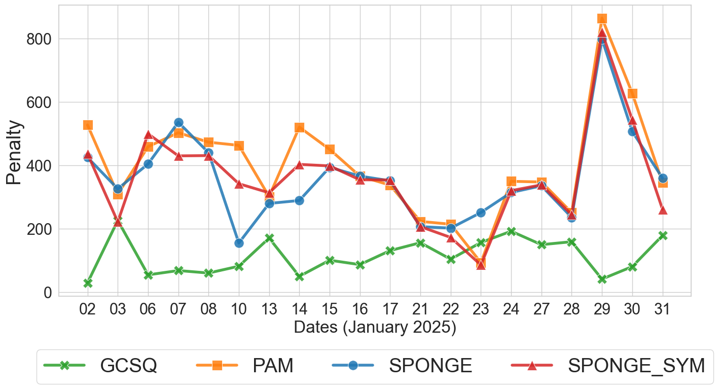 Penalty comparison across clustering algorithms over business days in January 2025 [1]
Results and Discussion
The results demonstrate clear advantages of GCS-Q over classical baselines:
GCS-Q consistently achieves the lowest penalty across nearly all trading days, often by a large margin. On some days, GCS-Q’s penalty is an order of magnitude lower than PAM’s.
PAM performs worst overall, which is expected since it relies on the lossy distance transformation and a centroid-based objective that does not align with the correlation clustering goal.
SPONGE and SPONGE_sym perform moderately, benefiting from their ability to handle signed graphs. However, they struggle because they are designed for sparse graphs with weights in ${-1, 0, +1}$ and balanced cluster sizes — conditions rarely met in financial correlation data with continuous weights and heterogeneous cluster structures.
GCS-Q determines $k$ dynamically, typically finding 2–11 clusters depending on the day’s correlation structure, while the classical methods are constrained to the $k$ estimated by the spectral gap heuristic.
Why Does GCS-Q Win?
- No information loss: GCS-Q works directly on the signed correlation matrix without any distance transformation.
- Exponential search space: At each bipartition step, the quantum annealer explores $\mathcal{O}(2^n)$ possible binary assignments simultaneously.
- Autonomous $k$ selection: The stopping criterion automatically identifies when further splitting would reduce clustering quality.
- Robustness to heterogeneous cluster sizes: Unlike classical methods that assume approximately equal-sized clusters, GCS-Q handles skewed distributions naturally.
Hardware Details
The QUBO subproblems are solved on the D-Wave Advantage_system5.4 annealer, which comprises 5,614 physical qubits and 40,050 couplers arranged in a Pegasus topology. Despite hardware noise and cloud latency (the dominant bottleneck due to remote access), GCS-Q delivers superior solution quality. Clustering 50 assets takes approximately a few minutes, with per-QUBO solve times capped at 1 second.
Scalability
GCS-Q has been validated on up to 170 fully connected assets with $k=10$ — the practical limit for fully dense graphs on current D-Wave hardware. Sparser correlation structures would allow scaling to even larger portfolios. Future hardware topologies (e.g., D-Wave Zephyr with higher connectivity) are expected to push this limit further.
Broader Context
This work is presented in two complementary papers:
QUEST-IS 2025 [1]: Focuses on the financial application — asset clustering using real Yahoo Finance data. Demonstrates that GCS-Q outperforms PAM, SPONGE, and SPONGE_sym in terms of structural balance penalty on real stock data.
IEEE QAI 2025 [2]: Provides the general correlation clustering framework, adapting GCS-Q for arbitrary signed graphs. Benchmarks against $k$-Means, PAM, DIANA, Spectral, and Hierarchical clustering on synthetic balanced graphs and real hyperspectral remote sensing data.
Together, these works demonstrate that GCS-Q achieves quantum advantage in solution quality using real quantum hardware, validated on both synthetic and real-world datasets. This marks a concrete step toward near-term quantum utility for graph-based unsupervised learning.
Conclusion
Classical clustering methods were designed for a world of positive-definite distances and spherical clusters. Financial correlation matrices do not live in that world — they are signed, dense, and rarely structurally balanced. GCS-Q bridges this gap by formulating clustering as recursive minimum-cut optimization on the native signed graph, leveraging quantum annealing to explore the exponentially large solution space efficiently.
If you work with correlation-based data — whether in finance, bioinformatics, or remote sensing — this pipeline offers a principled, quantum-enhanced alternative to classical heuristics. The code is open-source and ready to run.